Programming Homework 2
Submission instructions: Following the poll, the option that was upvoted was the markdown one. So, please use your Python notebook for your programming and written answers. This is done by including so-called “text cells” or “markdown cells” in your Python notebook. You can just type in your answers in these cells as text. So you have one document (the notebook) with all your answers.
To submit, save the notebook as PDF and submit this PDF as your answer. We will also accept other formats for your submission if this does not work for you. At the end however, you need to have a single PDF file for submission. That’s the only option available in gradescope.
Example of markdown cell:

Editing a markdown cell to enter your answer:

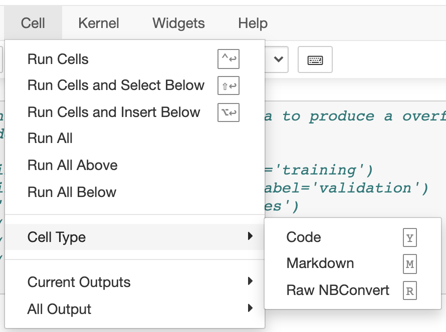
Converting a cell to a markdown cell:
In this homework, you will practice implementing and training simple neural networks using tensorflow and keras. We will first use the Higgs Dataset, a Physics Science dataset published by UC Irvine.
Source of the dataset: Daniel Whiteson, daniel ‘@’ uci.edu, Assistant Professor, Physics & Astronomy, Univ. of California Irvine. Reference: Baldi, P., P. Sadowski, and D. Whiteson. “Searching for Exotic Particles in High-energy Physics with Deep Learning.” Nature Communications 5 (July 2, 2014).
Data set information: the data has been produced using Monte Carlo simulations. The first 21 features (columns 2-22) are kinematic properties measured by the particle detectors in the accelerator. The last seven features are functions of the first 21 features; these are high-level features derived by physicists to help discriminate between the two classes.
Attribute information: The first column is the class label (1 for signal, 0 for background), followed by the 28 features (21 low-level features then 7 high-level features). For more detailed information about each feature see the original paper.
Our classification task is that given the 28 features, we want to predict whether the observation is a “signal” (class 1) or the background (class 0). Different activations, corresponding initialization schemes, and different optimizers will be discussed later in the course. For this homework, please use the ones specified in the questions. Keras documentations, and Google, will be helpful throughout this homework to understand the keras APIs.
You will find the starter code for this homework in the folder hw2-starter-code. The python dependencies required for this homework are listed in requirements.txt. If you are using Anaconda, you can install them by running pip3 install -r requirements.txt
Launch higgs.ipynb to get started. Before running the code, you need to download the dataset to your computer. Type this URL in your internet browser:
http://mlphysics.ics.uci.edu/data/higgs/HIGGS.csv.gz
Your browser should start downloading the file. The file size is 2.6 GB. It will take several minutes to download. Move this file to the directory containing the file higgs.ipynb for your homework.
The code for preprocessing dataset has been given to you and is at the beginning of higgs.ipynb.
- Build a model with a single fully connected hidden layer of size 32, using ReLU for activation and He normal for weight (kernel) initialization. Remember that the output layer doesn’t need activation. Compile the model with the Adam optimizer and use binary cross entropy as the loss function. Check out the keras documentation and guide to see how to specify them. Call the
summarymethod of the model to see its details.
Submission instructions: turn in the code in your notebook to perform the following:
- Build the model
- Compile the model
- Run
summary()and print the output
Answer the following question: how many trainable parameters does the model have?
Note on training: Take a look at the fit method to understand what arguments are available. In the solution set, we don’t specify anything other than the number of epochs, but you are free to experiment.
Calling fit multiple times doesn’t start training from scratch but continues from where it left off. So you can run fit multiple times to see how your model is progressively improving. To restart a training over from scratch, re-run the model creation function (e.g., model = tf.keras.Sequential()) to re-build the model. You can also save your model to be reloaded later.
Training neural networks can be difficult because you usually need to tune hyperparameters. The learning rate controls the trade-off between training speed and quality of convergence. For models in this homework, a learning rate on the order of $10^{-3}$ should work. You can experiment with different learning rates to find one that gives you the best convergence.
The learning rate can be changed using model.optimizer.learning_rate.assign(new_lr). You are also free to use other approaches, such as using a scheduler for learning rate. Note the potential danger of observing a premature convergence you train with a small learning rate.
For each training question, we will give reference numbers for epochs and loss, but you won’t necessarily get the same results since it depends on initialization. You are, however, expected to train your models until certain behaviors occur, which will be specified in questions.
Every call to the fit method returns a history object, which contains useful information such as the loss values of the training session. You can plot the loss to see if it is decreasing, and print the average for say, the first and last 10 losses. We provided a print_dot callback function that you can use in conjunction with setting the verbose option to 0 in fit. This reduces the amount of data printed in the notebook output cell. The print_training_info function can be used to print the final loss given the history object.
- Train your model using
x_train(input) andy_train(output) until the loss plateaus or decreases very slowly. For reference, we get a training loss less than 0.55 after ~400 total epochs. The loss was around 0.5 after 1,000 epochs.
Submission instructions: turn in the code in your notebook to train the model. In addition, answer the following questions:
- Report the learning rate you used
- Report the final loss
- Plot the loss function showing its convergence
Next, we will look at the problem of overfitting using training and validation data.
- Before we start, let us make sure our training and validation split is reasonable. Using numpy’s norm function, compute the l2 norm for each data point (row) in x_train and x_val. Plot the histograms for the norms of two data sets using plt’s hist function. Inspect the two distributions to make sure they are reasonably similar. You may use the following syntax for plotting:
plt.hist(data, n_bins, density=True)
https://matplotlib.org/3.1.1/api/_as_gen/matplotlib.pyplot.hist.html
density=True normalizes the data so that the area (or integral) under the histogram sums to 1.
Submission instructions:
- Turn in the code to compute the histogram
- Turn in your plot of the histogram
In addition, comment on the two distributions.
-
Build a new model with two hidden layers, both of size 32. Submission instruction: turn in the code of building and compiling the model in your notebook.
-
Train the model with (x_train, y_train) as training data and (x_val, y_val) as validation data. You should start to see a clear overfit behavior at some point: the training loss decreases, but the validation loss increases. Train the model to convergence to ensure you have an overfitted model. For reference, we start to see overfit after ~100 epochs; the final losses are 0.3~0.4 and > 1.0 for training and validation, respectively.
Submission instructions: turn in the code to train the model
In addition, turn in the following written comments:
- Report your final losses
- Plot the losses showing the overfit behavior
-
In your own words, explain what the model is doing when the training loss decreases, but the validation loss increases. What is the implication of this on the ability for the model to make a prediction on unseen data?
-
We will counter the overfit problem with l2 regularization. Build a new model with the same architecture as the last one, but with l2 regularization added to the weights (kernels) only, not the biases. The value of the regularization hyperparameter
lin the regularizer will need to be tuned. You can also experiment with using differentlin different layers. Submission instruction: turn in the code in your notebook. -
Tune your regularization hyperparameter(s) by training the models with different
l. We want both errors to stabilize without the validation error increasing in the process; and the optimal value is the smallestlthat gives this behavior. Thislshould also give you the smallest validation error. For reference, our training and validation loss converge to ~0.57 and 0.7, respectively, after ~1k total epochs. We recommend experimenting with l in the [$10^{-2}$, $10^{-5}$] range.
Submission instruction: turn in the code used to train the model.
In addition, turn in the following written comments:
- Report the final
lvalue(s) you tuned - Report the final training and validation losses
- Include a plot showing how the errors stabilize to the reported values.
- In your own words, explain how l2 regularization counters overfitting.
One of the key signs of an overfitted model is that the model is very sensitive to noise in the input or to the specific choice of training points. Generally speaking if one considers a function $f(x)$, the sensitivity can be estimated by computing
\[\int \left( \frac{df}{dx} \right)^2 p(x) \, dx = E((f')^2)\]where $p(x)$ is the probability density function of $x$ and $E$ denotes the expectation. To estimate this quantity, we can add some noise $r$ to the input $x$. Let us assume that we add a small amount of noise such that
\[f(x + r) \approx f(x) + \frac{df}{dx} r\]to first-order. The noise $r$ is a normal random variable, with mean 0 and variance $\sigma^2(r)$, which is uncorrelated with $x$. The variance of $f(x+r)$ is equal to
\[\sigma^2(f(x+r)) = \sigma^2(f(x) + f'(x) r) = \sigma^2(f) + \sigma^2(r) E((f')^2)\]We see that when the noise has variance 0 (i.e., $\sigma^2(r)=0$), we get $\sigma^2(f)$ as expected. As the variance of $r$ increases, the variance of $f(x+r)$ increases linearly with slope $E((f’)^2)$. This slope represents how sensitive the function $f$ is to changes in the input $x$.
Numerically, this can be estimated by adding some noise $r_i$ drawn from a normal distribution to each input variable $x_i$ and computing the standard deviation of the output $f(x_i + r_i)$. As we vary the variance of $r_i$, the rate of change of $\sigma^2( f(x_i + r_i) )$ measures the sensitivity.
Below we will compare two different models that have comparable accuracies, but different sensitivities. In that case, the model that has the largest variance for $f(x+r)$ is the most sensitive one.
-
Let’s compare our overfitted and regularized models by investigating how sensitive they are to input noise. You can generate Gaussian noise using np.random.normal. We will generate noise with 0 mean and standard deviations of [0.1, 0.2, 0.3, 0.4, 0.5]. For each standard deviation value, repeat 10 times the following:
- Generate noise; add the noise to x_val to generate a perturbed input (don’t modify x_val itself).
- Compute the predictions for the perturbed input using both models.
- Compute the standard deviation for the two predictions.
- Compute the error (see below for details on how to do that) for the two predictions using y_val as true value.
Average these results over your 10 runs. Repeat for all noise levels.
To use your model to make a prediction, use (predict):
model.predict(x_input)
To use your model to evaluate its accuracy, use (evaluate):
model.evaluate(x_input, y_output, verbose=0)[1]
evaluate returns the loss value & metrics values for the model. We use [1] at the end to get the metrics value only. In our example, our metric is accuracy which calculates how often predictions equal labels. This is a number between 0 and 1. In this case we can define the error as:
1 - model.evaluate(x_input, y_output, verbose=0)[1]
This is always a positive number, between 0 and 1.
Code submission instruction:
- Turn in the code used to compute the standard deviation vs noise
- Turn in the code used to compute the classification error in your model vs noise
In addition, turn in the following:
- Plot the mean standard deviation of the output vs the standard deviation in the input noise
- Plot the classification error vs the standard deviation in the input noise
- Qualitatively, based on the plots, comment on the two models’ sensitivity to the input noise.